What is 'Custom Format' ?: Microsoft Office Excel provides many built-in number formats, but in some cases they do not meet our needs, we can customize a built-in number format to create our own.
Why 'Custom Format' and not 'Conditional Formatting'?: because to cure 'Common Cold' we go to doctors not surgeons. Exactly, when there is a simple and robust way then why to go otherwise. There are many benefits of using custom format including these:
1. Less overhead than Conditional Formatting.
2. Values can be used easily in formulas (Less manipulation required).
3. Charts looks better with custom colored labels/axis.
4. Works on all versions of Excel.
and many more which you can figure out using your innovative mind after reading this article.
How to apply 'Custom Format'?
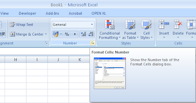
Step 1: Open 'Format Cells' dialog box using any of your favorite options:
i) Ctrl + 1
ii) Right Click --> 'Format Cells'
iii) Home --> Numbers (Bottom right arrow) - See the pic

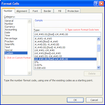
Step 2: Now click on 'Custom' and start typing your 'Custom Format' code.

'Custom Format' coding: A number format can be divided in 4 parts by semicolons. Each part is an individual number format. The first applies to positive numbers, second to negative numbers, third to zeros, and the fourth to text (This is by default or we can define this too).
So we can represent the custom format like this.
Positive Numbers ; Negative Numbers ; Zeroes ; Text
Of course we can skip whatever we want to as per the requirements and use it like any of this:
Positive Numbers;;Zeroes;Text
Positive Numbers;Negative Numbers;;Text
Positive Numbers;Negative Numbers;Zeroes
etc etc.
Even we don't have to include all semicolons. If we specify only 2 code sections for our custom number format, the first section is used for +ve numbers and zeros, and the second section is used for -ve numbers. If we specify only one code section then it is used for all numbers.
Whenever we skip custom format for a particular type, General format is assumed for the same. This technique comes very handy when we want to hide the values with no data in charts. We can use <any format>;;; to achieve this. For e.g.
General;;;
0%;;;
#.##;;; etc. etc.
Examples:
Let's move with some examples of various data. Essentially, examples makes this subject simple.
I - BASIC EXAMPLES
II - INTERMEDIATE EXAMPLES
III - ADVANCED EXAMPLES
By now either you have completely understood the Number/Date/Text Formatting using CUSTOM Format or not. In any case I'm sure that you'll be looking for more detailed information. So we will now move on to theory of 'Custom' format.
Before that, I've some exercise questions for you - if you can do them you are genius dude. Try on your own and devote sometime before you google them. This will also help you learn limited theory (which you actually need rather than whole post).
I'm waiting for your responses in comments ;)
So here is some theory for you:
Why 'Custom Format' and not 'Conditional Formatting'?: because to cure 'Common Cold' we go to doctors not surgeons. Exactly, when there is a simple and robust way then why to go otherwise. There are many benefits of using custom format including these:
1. Less overhead than Conditional Formatting.
2. Values can be used easily in formulas (Less manipulation required).
3. Charts looks better with custom colored labels/axis.
4. Works on all versions of Excel.
and many more which you can figure out using your innovative mind after reading this article.
How to apply 'Custom Format'?
Step 1: Open 'Format Cells' dialog box using any of your favorite options:
i) Ctrl + 1
ii) Right Click --> 'Format Cells'
iii) Home --> Numbers (Bottom right arrow) - See the pic

Step 2: Now click on 'Custom' and start typing your 'Custom Format' code.

'Custom Format' coding: A number format can be divided in 4 parts by semicolons. Each part is an individual number format. The first applies to positive numbers, second to negative numbers, third to zeros, and the fourth to text (This is by default or we can define this too).
So we can represent the custom format like this.
Positive Numbers;;Zeroes;Text
Positive Numbers;Negative Numbers;;Text
Positive Numbers;Negative Numbers;Zeroes
etc etc.
Even we don't have to include all semicolons. If we specify only 2 code sections for our custom number format, the first section is used for +ve numbers and zeros, and the second section is used for -ve numbers. If we specify only one code section then it is used for all numbers.
Whenever we skip custom format for a particular type, General format is assumed for the same. This technique comes very handy when we want to hide the values with no data in charts. We can use <any format>;;; to achieve this. For e.g.
General;;;
0%;;;
#.##;;; etc. etc.
Examples:
Let's move with some examples of various data. Essentially, examples makes this subject simple.
I - BASIC EXAMPLES
| COMMENTS | TO DISPLAY | AS | USE THIS |
| Leading Zeros | 26 | 0026 | 0000 |
| Phone Number | 9999505853 | 999-950-5853 | 000-000-0000 |
| Day of the Date | 22/11/1994 | Saturday | dddd |
| Month of the Date | 22/11/1994 | May | mmmm |
| Comma Place holder | 23456789 | 23,456,789 | #, ### |
| Currency | 2605.5 | € 2,605.50 | € #,###.00 |
II - INTERMEDIATE EXAMPLES
| COMMENTS | TO DISPLAY | AS | USE THIS |
| Decimal | 2.1 | 02.10 | 00.00 |
| Positive (Green) | 2605 | 2,605 | [Green]$#,##0;[Red]$#,##0 |
| Negative (Red) | -1984 | -1,984 | |
| Trailing Dots | eXceLitems | eXceLiTems.......... | @*. |
| Scientific Notation | 123450 | 12.345E+04 | ##.000E+00 |
| 123.450E+03 | ###.000E+00 | ||
| 1.235E+05 | 0.000E+00 | ||
| Round Off to 1000th | 26051984 | 26052 | #, |
| Align Decimals | 26.051 | 26.051 | ???.??? |
| 512.65 | 512.65 | ||
| 3.6 | 3.6 |
III - ADVANCED EXAMPLES
| COMMENTS | TO DISPLAY | AS | USE THIS |
| Prefix Text | 12 | EMP0012 | "EMP" 0000 |
| Suffix Text | 125 | 1,250 lbs. | #,##0 "lbs." |
| Textual Currency | $5.75 | 5 dollars and .75 cents | 0 "dollars and" .#0" cents" |
| Positive (Green) | 512 | 512.00 | [Green]#,##0.00; [Red](#,##0.00);[Blue]"Zero" |
| 0 as Zero (Blue) | 0 | Zero | |
| Negative (Red) | -652 | (652) | |
| Varying Decimal Digits | .023 | .023 | [RED][<0.1]0.000; [Blue][<1]0.00;[Green]0.0, |
| .23 | .23 | ||
| 2.3 | 2.3 | ||
| Elapsed Time (Hours & Minutes) | Formula with Time difference | 1:02 | [h]:mm |
| Elapsed Time (Mins. & Secs.) | 62:05 | [mm]:ss | |
| Elapsed Time (Secs.&Hundredths) | 3725.62 | [ss].00 | |
| Calculate Kilo(103) | 100000 | 100K | [>=1000]0,"K" |
| Calculate Mega(106) | 5000000000 | 5000K | [>=1000000]0,,"M";[>=1000]0,"K";0 |
| Align Fractions | 6.25 | 6 1/4 | # ???/??? |
| 5.43 | 5 43/100 | ||
| 7.75 | 7 3/4 |
By now either you have completely understood the Number/Date/Text Formatting using CUSTOM Format or not. In any case I'm sure that you'll be looking for more detailed information. So we will now move on to theory of 'Custom' format.
Before that, I've some exercise questions for you - if you can do them you are genius dude. Try on your own and devote sometime before you google them. This will also help you learn limited theory (which you actually need rather than whole post).
| COMMENTS | TO DISPLAY | AS | USE WHAT |
| Negative Number | -123000 | (123K) | ? |
| Date | 26/05/1984 | Sat, May '84 | |
| Currency | 6.56 | £7 | |
| Labels | 25 | 25 feet | |
| Round off to 1000000th | 987654321 | 988 |
I'm waiting for your responses in comments ;)
So here is some theory for you:
| Character | Used as/for |
| 0 (Zero) | This digit placeholder displays insignificant zeros if a number has fewer digits than there are zeros in the format. For example, if you type 2.6, and you want it to be displayed as 2.60, use the format #.00 |
| # (Hash) | This digit placeholder follows the same rules as the 0 (zero). However, Excel does not display extra zeros when the number that you type has fewer digits on either side of the decimal than there are # symbols in the format. For example, if the custom format is #.##, and you type 8.3 in the cell, the number 8.3 is displayed and 2.657 is displayed as 2.66 |
| ? (Ques. Mark) | This digit placeholder follows the same rules as the 0 (zero). However, Excel adds a space for insignificant zeros on either side of the decimal point so that decimal points are aligned in the column. For example, see above(Last Intermediate Example) |
| . (dot/period) | This digit placeholder displays the decimal point in a number. |
| Color Codes | These are the only approved colour codes. [BLACK] or [Green] or [White] or [Blue] or [Magenta] or [Yellow] or [Cyan] or [Red] |
| Specify Conditions | To specify number formats that will be applied only if a number meets a condition that you specify, enclose the condition in square brackets. The condition consists of a comparison operator and a value. For example, see 2nd intermediate or 5th, 6th, 10th and 11th advanced examples. |
| E (E+/E-) | Exponential Notation/Scientific Notation: Displays a number in scientific (exponential) format. Excel displays a number to the right of the "E" or "e" that corresponds to the number of places that the decimal point was moved. For example see 5th Intermediate example. |
BONUS VBA MACRO: Excel 2003 Style menu in Excel 2007 / 2010
Are you going for an interview ?
3 things to remember before Excel VBA Interview
50 Excel VBA Interview questions
or looking for a job ?
Excel, Access, SQL, VBA, MIS, Reporting and Data Analysts Jobs
3 things to remember before Excel VBA Interview
50 Excel VBA Interview questions
or looking for a job ?
Excel, Access, SQL, VBA, MIS, Reporting and Data Analysts Jobs

Comments
ddd, mmmm, ‘yy
“$”0
I couldnt figure it out
#,,
////////////
BTW, I have another question for you.
Is there any chance I could reformat "32187.56892" into 32200?
Any other answer instead of #,"200"?
instead of "$"0, you need to use £0 (£ can be obtained using ALT+0163)
and the fourth is 25" feet".
and I like your question, unfortunately I don't have answer for the same. I would be happy, if you have :)
Hi,
I am using the excel 2007 and automating through Microsoft Visual Foxpro 9. Every thing goes fine except the numberformat property. I want the digits should group in 2 instead of 3.
1.) Positive number
figure 1234763466.98
applied numberformat "##,##,##,##,###.#0;-##,##,##,##,###.#0;;"
expected display 1,23,47,63,466.98 (2 digits should be grouped)
actual display 1,234,763,466.98 (3 digits are grouped)
2.) Negative number
figure -1234763466.98
applied numberformat "##,##,##,##,###.#0;-##,##,##,##,###.#0;;"
expected display -1,23,47,63,466.98 (2 digits should be grouped)
actual display -1,234,763,466.98 (3 digits are grouped)
3.) Number with no decimal
figure 1234763466 (No decimal here, but .00 is expected at end in excel)
applied numberformat "##,##,##,##,###.#0;-##,##,##,##,###.#0;;"
expected display 1,23,47,63,466.00 (2 digits should be grouped)
actual display 1,234,763,466.0 (3 digits are grouped)
4.) Zero
figure 0 (it is working fine.)
applied numberformat "##,##,##,##,###.#0;-##,##,##,##,###.#0;;"
expected display ""
actual display ""
5.) Number with one decimal
figure 12347.3 (one digit after decimal, it is working fine.)
applied numberformat "##,##,##,##,###.#0;-##,##,##,##,###.#0;;"
expected display 12,347.30
actual display 12,347.30
if I supply the values as characters like "1,23,47,63,466.00" to the cells then the excel display is okay but the formulas where i have to sum them does'nt work. they yeild result like #value.
What I want is the step 1,2,3 should also produce the expected display without changing its behaviour in step 4 and 5. The summation (formulas) should also work.
thanking you in advance.
from
dharm.software@gmail.com